Modelling Probability of Loan Default

When banks and other financial institutions evaluate a loan request, they must ascertain the risk of default. Defaults can be very costly to banks and predictive analytics can be deployed to help banks make the right decisions. This project involves using a past Kaggle competition to model default of a customer based on many different features.

Data Exploration

The dataset comprises over 300,000 customers with over 100 features; it is quite a large dataset packed with data. Let's try to make sense of it. It gives demographic and financial information of a customer and then says if he/she defaulted on a loan.

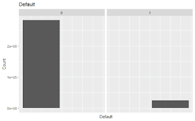
Let's first get a broad-level overview of the fraction of defaults.

The bank issues both cash loans and revolving loans. The latter are flexible loans and are rather open-ended. Let us see how default rates vary based on the type of loan.

It seems that a smaller proportion of revolving loans, as opposed to cash loans, suffer from default. This makes intuitive sense as revolving loans are more likely to be issued to more trustworthy borrowers.

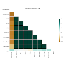
We want to identify if there is any relation between income, the amount of credit, and default.

Interestingly, there does not appear to be any such relationship. Here, the red circles are customers who defaulted and they seem to be well mixed-in with the blue circles, those who did not default.

Data Cleaning

I convert some of the categorical variables, such as gender and binaries for car and home ownership to numeric to make analysis easier.

It is important to explore various columns to check for anomalies.

The age column looks like this:

 Min. 1st Qu.  Median    Mean 3rd Qu.    Max. 

 -25229  -19682  -15750  -16037  -12413   -7489 

Clearly, this needs to be fixed. We just need to divide by -365 to get the age in years. We then round down to get the age in years.

The column for days employed is also anomalous. There is one outlier value which has been inputted for many records.

Test data

We split the data into the training set, which will be used to create the models, and the best model will be decided based on how well it predicts the test data. The training data comprises the first 70% of the data (the first 215257 records) and the remaining 30% is the testing data.

Model 1: Logistic Regression
My first model is logistic regression. The features selected along with their coefficients are at the end of the post as they look quite ugly...

While most variables are significant, this model is clearly not optimal, given the R-squared value of just over 5%.  I use this model to predict the test data (the remaining 30% of our observations).

Explaining the Variables
Most, but not all, variables included in the model are statistically significant, at least at the 10%. The initial variables include the type of loan and a binary for car ownership, which are as expected. Interestingly, home ownership was not significant as a determinant of the probability of default, when other factors are accounted for.

With regards to family status, the baseline was civil marriage and it seems that every other family profile has a lower probability of default on average than civil marriage. The HOUR_APPR_PROCESS_START variable refers to the time the loan application was initiated, presumably online, with 0 (12AM) as the baseline. It is interesting to note that this variable is significant for almost all hours; it appears that those who begin their applications at midnight are the riskiest borrowers.

Many occupation factors are significant; here, the baseline is the Unknown category, and relatively higher-paying occupations are less risky. There is likely a correlation with income here, and since income was insignificant, it is not in the model.

Location variables are also important here; those who live, work, and register their application for the loan in the same city are the safest applicants.

There is no information on what each document is so it is impossible to make any conclusions on what the documentary evidence of a loan application can tell about the applicant's probability of default.

The older the person is and the longer they have worked, the safer they are. There is also an interaction for age and years worked included to highlight the non-linearity.

Performance of Model
Given the low explanatory power of the model, it is not surprising that the model did not perform very well on the test data. This graphic conveys this finding.

Model 2: K-Nearest Neighbours
There are alternatives to logistic regression which can be tried, for example, k-nearest neighbours.
I use the same variables as in the above case, however, all are now numerically coded.

Using the 20 nearest neighbours to predict the outcome, I predict whether a customer will default based on the given features. This is the outcome contingency matrix.

                                   Actual_Outcome
Predicted_Outcome           0          1
                0                  63687      5492
                1                  5160          966

In this case, k-nearest neighbours has also not given very good results. In particular, there is a very high false positive rate. Of all the predicted customer defaults, only 15.8% of customers actually default. Meanwhile, of all the customers who are not predicted to default, 7.9% actually default; this is not a good result given the very low base rate of non-defaulters.

Conclusion
In this case, neither logistic regression nor k-nearest neighbours have provided satisfactory results. This could be due to a variety of reasons. One, the data may not be relevant enough for the purpose of predicting the probability of default. A second reason could be improper variable selection from the available data.

This exercise gives insight into the complexity of tasks for a financial institution while deciding whether to issue a loan. There are many factors which can influence a customer's probability of default and banks have to maintain lots of data to build reliable models to use for their decision-making.

Appendix: Coefficients from the Regression
(Intercept)
-0.79595
NAME_CONTRACT_TYPERevolving loans***
-0.18317
FLAG_OWN_CAR***
-0.26606
FLAG_OWN_REALTY
-0.01833
REGION_RATING_CLIENT***
0.355928
FLAG_WORK_PHONE***
0.258398
AMT_CREDIT***
2.79E-06
AMT_ANNUITY***
1.11E-05
AMT_GOODS_PRICE***
-3.57E-06
NAME_FAMILY_STATUSMarried***
-0.13747
NAME_FAMILY_STATUSSeparated
-0.04431
NAME_FAMILY_STATUSSingle / not married
-0.00917
NAME_FAMILY_STATUSWidow***
-0.29511
factor(HOUR_APPR_PROCESS_START)1.
-1.33273
factor(HOUR_APPR_PROCESS_START)2.
-0.92361
factor(HOUR_APPR_PROCESS_START)3*
-1.21312
factor(HOUR_APPR_PROCESS_START)4*
-1.17613
factor(HOUR_APPR_PROCESS_START)5*
-1.09525
factor(HOUR_APPR_PROCESS_START)6*
-0.99523
factor(HOUR_APPR_PROCESS_START)7*
-1.01898
factor(HOUR_APPR_PROCESS_START)8*
-1.03462
factor(HOUR_APPR_PROCESS_START)9*
-1.06499
factor(HOUR_APPR_PROCESS_START)10*
-1.08422
factor(HOUR_APPR_PROCESS_START)11*
-1.0546
factor(HOUR_APPR_PROCESS_START)12*
-1.06202
factor(HOUR_APPR_PROCESS_START)13*
-1.07317
factor(HOUR_APPR_PROCESS_START)14*
-1.06996
factor(HOUR_APPR_PROCESS_START)15*
-1.06118
factor(HOUR_APPR_PROCESS_START)16*
-1.12422
factor(HOUR_APPR_PROCESS_START)17**
-1.2677
factor(HOUR_APPR_PROCESS_START)18*
-1.15939
factor(HOUR_APPR_PROCESS_START)19*
-1.02128
factor(HOUR_APPR_PROCESS_START)20*
-1.1636
factor(HOUR_APPR_PROCESS_START)21*
-1.24743
factor(HOUR_APPR_PROCESS_START)22
-0.8558
factor(HOUR_APPR_PROCESS_START)23
-1.16614
FLAG_CONT_MOBILE.
-0.35471
FLAG_PHONE***
-0.10984
CNT_FAM_MEMBERS
0.001569
OCCUPATION_TYPEAccountants***
-0.25952
OCCUPATION_TYPECleaning staff*
0.133099
OCCUPATION_TYPECooking staff*
0.115596
OCCUPATION_TYPECore staff***
-0.15884
OCCUPATION_TYPEDrivers***
0.336836
OCCUPATION_TYPEHigh skill tech staff**
-0.163
OCCUPATION_TYPEHR staff
-0.0928
OCCUPATION_TYPEIT staff
-0.02068
OCCUPATION_TYPELaborers***
0.21998
OCCUPATION_TYPELow-skill Laborers***
0.534507
OCCUPATION_TYPEManagers
0.02606
OCCUPATION_TYPEMedicine staff*
-0.11466
OCCUPATION_TYPEPrivate service staff*
-0.24476
OCCUPATION_TYPERealty agents
-0.15031
OCCUPATION_TYPESales staff
0.008537
OCCUPATION_TYPESecretaries
-0.14882
OCCUPATION_TYPESecurity staff***
0.244169
OCCUPATION_TYPEWaiters/barmen staff
0.12137
LIVE_CITY_NOT_WORK_CITY*
0.240491
REG_CITY_NOT_WORK_CITY***
0.196464
FLAG_DOCUMENT_3***
0.219586
DEF_30_CNT_SOCIAL_CIRCLE***
0.210821
FLAG_DOCUMENT_2***
2.853055
FLAG_DOCUMENT_5**
0.227776
FLAG_DOCUMENT_13**
-0.61187
FLAG_DOCUMENT_11**
-0.39757
FLAG_DOCUMENT_14***
-0.92517
FLAG_DOCUMENT_15*
-0.91468
FLAG_DOCUMENT_16***
-0.60078
FLAG_DOCUMENT_18***
-0.4145
AGE***
-0.01692
YEARS_WORK***
-0.06549
UNACCOMPANIED**
0.0732
HIGHER_ED***
-0.41263
YEARS_LAST_PHONE_CHANGE***
-0.07162
ACADEMIC_DEGREE.
-0.97827
FLAG_OWN_CAR:FLAG_OWN_REALTY**
0.083924
LIVE_CITY_NOT_WORK_CITY:REG_CITY_NOT_WORK_CITY**
-0.33224
AGE:YEARS_WORK***
0.000624

Source of dataset from kaggle - https://www.kaggle.com/c/home-credit-default-risk/data