Investigating House Prices

Having now learnt a variety of machine learning models, as well as evaluative methods, it was time for some light practice using an old Kaggle dataset on house prices. Predicting house prices have a variety of applications from prospective buyers estimating the price of a house based on desired features to homeowners who wish to value their house before selling. While the entire analysis was carried out in R, I did a few cleaning bits in Python too to gain further practice.

Data Exploration
The training dataset is quite small, with only 1460 observations and about 79 variables. These variables included a variety of salient features about houses, including the neighbourhood, square footage, details on the number of rooms, whether the house has a fireplace, pool, garage and so on, as well as the age, and so on.

Let's first begin by exploring the data.

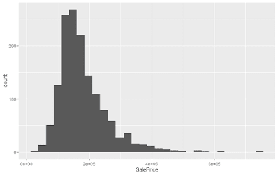Here is the distribution of house prices. We can see that the distribution is skewed to the right, with most houses around the $200,000 mark.










As I learn about data cleaning, one of the things I have begun to appreciate a lot is the various ways to deal with missing values. This dataset contained a significant number of missing values, whose relationships can be visualised:

We can see that there are many missing values and there are also patterns in which data is missing across columns. A closer analysis reveals strong relationships of missing values among variables relating to Garage, Basement, and so on.

What we can gather from this is that houses without a pool, or a fence, and so on have NA values for those respective columns. Therefore, in cases of factor variables (such as pool quality), I replace all NAs with the string NA, and treat those without a pool, or a fence, and so on, as a factor in its own right. Columns with quantitative values are imputed to 0; for example, houses without a front lot have a front lot with area 0, therefore, I replace the NAs with 0 in the respective column.

I delete the Alley and ID columns as they do not add anything meaningful to the data. After taking care of all missing values, I do not have to delete any observations.

Data Transformations
There are columns relating to the year of sale, year of construction, and so on. The latest year in all such columns is 2010, therefore, I assume that this data relates to 2011 data. I convert all year fields to time fields, so a house built in 2010 is now stated as being 1 year old. This transformation prepares the data for modelling.

Clustering via K-Means
Rather than looking at data one variable at a time, it makes sense to look at data grouped by certain variables, and use a clustering algorithm to create like groups and reduce the number of features to work with.

I am interested in how houses differ in their total area and area of certain rooms, and how this has varied over time. Therefore, I cluster houses by their lot area, basement area, living area, garage area, and age.

We find that the HDIC is minimum at 4 clusters, therefore, we choose to segment our houses into 4 groups.

Cluster 1 refers to older houses with  huge lots and basements and relatively large garages and living areas. Cluster 2 refers to new houses which are relatively average-sized in all dimensions. Cluster 3 are not very different from Cluster 2 houses, just bigger in all respects, especially with respect to their lot area. Finally, Cluster 4 houses are the oldest of the lot and smaller than average, and may lack a garage and/or a basement.

Here, we can see how the garage area and living area of the house relate, and the clusters to which the houses belong.

Dimension Reduction Through Principal Component Analysis (PCA)
While clustering helped us group houses by similar attributes, we still have too many variables and need a more systematic approach to reducing the number of features in our model. Enter PCA, which identifies the variables which most explain the variance in Sales Price. The technique creates components, each of which is a basket of variables stacked in with varying weights, which together explain our data.

The first principal component explains much of the variation in the Sales Price, and looking at the top 3 components helps explain the vast majority of the variance.

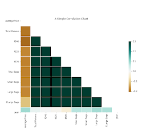
Upon considering the most important features in each of the components, and identifying any correlations among those features, we can begin developing models.




Model 1: Regression Tree
Using all the variables in the data, I created the regression tree.

The tree is hard to read, however, it does indicate that the clusters we created (known as colorcluster) is an important variable, as it is the first one by which houses are categorized. The tree achieved an in-sample R-square of 76.6%.

What is very useful about the tree model is that it tells us which variables are the most important in the data. This, along with the principal components developed earlier, informs the linear regression model run, which achieved an in-sample R-square of 79.3%.

Finally, I used an ensemble model, the random forest. Developing the random forest required much more care as there is a limit to the number of factors it can take as input. Iterating over several models, my random forest model achieved an in-sample R-square of 86.4%.

Evaluation
I carried out 10-fold cross-validation of the three models discussed above with the null model as a baseline. Here are the results from the evaluation:

The random forest model achieved the best average out-of-sample R-square of 86% while the corresponding numbers were 78.2% for linear regression and 68.7% for the tree. The random forest model is likely to be better suited to deploy to predict actual house prices. 

So What Determines House Prices?

According to the random forest model, the most important variables include those relating to the area of the living room, and first floor, as well as garage area. The cluster which associated the age and size of houses is also important as is the neighborhood. Interestingly, the age of the home also features among the most important variables.